Excel-User.com

Yes, that’s right! Today I’ve reached the (first) million pageviews since I’ve started, on May 2007. I want to thank you all for passing by. I hope that you continue to visit me and enjoying the work that I do here.

You can download the Microsoft Excel 2013 Quick Start Guide (aka “Cheat Sheet”) here:

http://officeimg.vo.msecnd.net/en-us/files/514/375/AF103733534.pdf

This is a great tool to help you get started with this new version of Excel.

You can also find the complete collection of Microsoft Office 2013 Quick Start Guides here:

http://blogs.msdn.com/b/mssmallbiz/archive/2013/02/06/complete-collection-of-microsoft-office-2013-quick-start-guides-cheat-sheets.aspx

First of all, if you want to install Office 2013, you will need either Windows 7 or Windows 8. Previous versions of Windows are not support.
When you install Office 2013, you can either do a side-by-side installation or upgrade from previous version.
If you do a side-by-side installation, you can run either Excel 2010 or Excel 2013 on the same machine.
If you upgrade, you can do a full upgrade or just remove one or more Office 2010 applications.
When you run the Office 2013 installer, you will need, as usual, to accept the license terms:

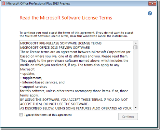
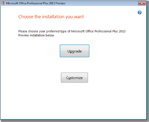
You then get the option to upgrade or customize your installation:

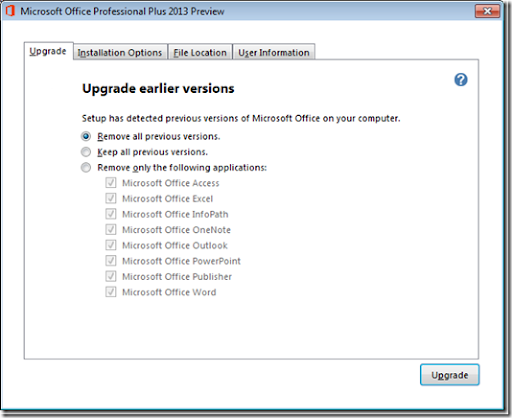
If you want to remove all previous versions, you should choose Upgrade. If you want to install Office 2013 side-by-side with Office 2010, you should choose Customize. You will then get this options:

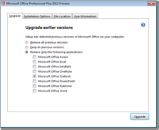
Here you can choose to remove all previous versions and do a full upgrade (first option “Remove all previous versions”, you can choose a side-by-side installation choosing the second option (“Keep all previous versions”) or remove one or more of the older Office 2010 applications by choosing the third option “Remove only the following applications”) and then ticking the applications that you want to remove. You have here a restriction that is Outlook 2013. You cannot have Outlook 2010 and Outlook 2013 on the same machine so you have to remove, at least, Outlook 2010 from the previous installation. So, to have a side-by-side installation of both Office 2010 and Office 2013 on the same machine, you should select the third option and tick “Microsoft Office Outlook” option, like this:

After the installation, the existing Excel files will open on the new Excel 2013 version. If you want to open file on the Excel 2010 version, you should open Excel 2010 and then open the files by going to the File-Open menu.

My article written for Microsoft Office Blog in 2012 about “Using multiple criteria in Excel Lookup formulas” was recognized as the number one on the “Top 5 posts about the current Excel” category.
I’m very happy to see that my work with Excel is recognized by the community. Hope to continue writing articles to show you how you can improve your Excel skills.

I’ve tested the new online version of the uCertify PrepKits that I’ve used before and that I’ve reviewed here. This new online platform means that you don’t need to install anything on your computer to start using the prep kits.

Some of the features of Online PrepEngine are:

• Complete location and device independence: Available online 24x7 or go mobile (supported on all major Smartphones and tablets)
• Digital book integrated with images, videos, audio, quizzes, flash cards, assessments, assignments, study notes and much more
• Powerful Analytics to track and gauge learning effectiveness for students, teachers and school administrators
• Self-Study or Teacher/Mentor assisted learning
• Student-Student & Student-Teacher Collaboration tools
• Customizable roles and access for students, TAs, teachers and administrators
• Simple, yet powerful teacher portals to customize courses, pre-assessments, tests and assignments
• Hassle free, highly available and scalable hosted solution

Additionally, there is another feature ‘Course Advisor’ which is a helpful tool for one who is confused to choose certification exam. This tool will help such person to choose certification based on his/her interested technology, experience level, and education.

As before, I found that this tool is extremely simple to use. I just logged in and went straight to the Courses area where I found the courses that I had available. I open the 77-888 (Microsoft Excel 2010 Expert) and I had many options to follow, like a “Pre-assessment”, where I had 15 question to test and assess my strengths & weaknesses, a “Practice” mode with 74 questions, a “Quiz” with 101 questions, “Flash Cards” with 89 flashcards as well as, among others, a “Final Test” to test your knowledge and make you a final test to see if you could pass the official exams.

The online platform has a good design and it’s very intuitive to use. You can find hundreds of courses and certifications here. The value of the kits remains very good and I think that it’s a good value for money if you’re thinking on going for any IT certification, I’m sure that you will find here the prep kit to help you train and test your knowledge

This article was originally written for the Microsoft Excel Blog. The purpose of this article is to show Excel users some technique’s, and Excel functions, that they can use to lookup up a value on a table, using more than one criteria. If you have only one criteria, it’s simple, you can use a plain VLOOKUP formula to do that. If you want to use more than one, then there are lots of ways of doing it, using several of Excel’s functions like VLOOKUP, LOOKUP, MATCH, INDEX, etc.

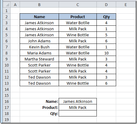
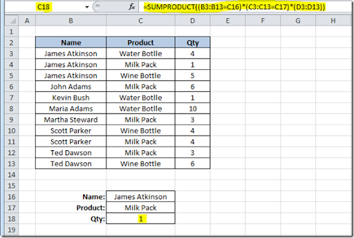
Let’s see a scenario where we want to use two criteria’s to return a value from a table. This is the data table that we have:

As you can see, we want to use a “Name” and “Product” criteria to return a “Qty” value on cell C18. We are going to look for the Name “James Atkinson” and the Product “Milk Pack” to return the Qty from the table. Because the value that we want to return is a number, we can use a simple SUMPRODUCT() formula in C18 cell, like this:

=SUMPRODUCT((B3:B13=C16)*(C3:C13=C17)*(D3:D13))

What this does is look on the range B3:B13 for the value on cell C16 and on the range C3:C13 for the value on cell C17 and where it finds both, return the value on column D, from the same row where it found both criteria’s. Here’s how it will look:

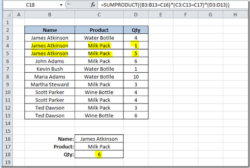
It is returning the value 1 that corresponds to the value on cell D4 because it found “James Atkinson” Name on row 4 and also “Milk Pack” on the same row, thus returning the value of column D from that row. Let’s just change value on cell C5 from “Wine Bottle” to “Milk Pack” to see what happens with the formula on cell C18:

Because our formula found two lines where both criteria’s were found, it is summing the values on column D on rows where they were found, giving us a Qty of 6.

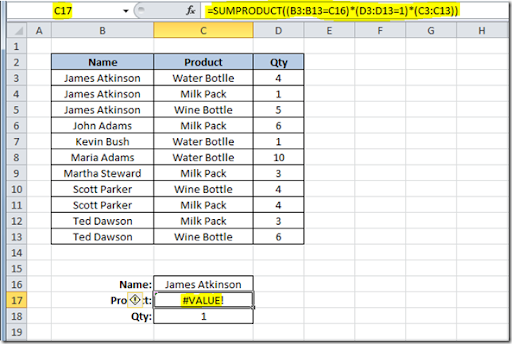
This technique cannot be used is we wanted to look for two criteria’s and return a text result. For instance, this, would not work:

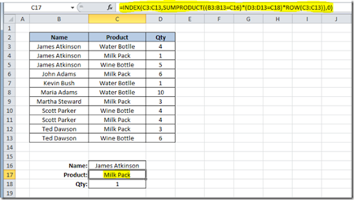
We are looking for the Name “James Atkinson”, where the Qty is 1 and we want to return the Product name that matches this two criteria’s. This formula would give us a #VALUE error! Instead we could use a formula using a combination of SUMPRODUCT, INDEX and ROW functions, like this:

=INDEX(C3:C13,SUMPRODUCT((B3:B13=C16)*(D3:D13=C18)*ROW(C3:C13)),0)

We use the SUMPRODUCT function to find out the row where both criteria’s are found and return the corresponding row number using the ROW function. Then we use it on the INDEX function to return the value on the array C3:C13 that is on the row number provided. The result will be like this:

This could also be done using a different technique. You could use this formula on cell C17:

=LOOKUP(2,1/(B3:B13=C16)/(D3:D13=C18),(C3:C13))

The result will be the same as the previous solution. What this formula does, is divide 1 by an array of True/False values (B3:B13=C16) and then by another array of True/False (D3:D13=C18). This will return 1 or a #DIV/0 error. Using 2 as the lookup value, then the match will be with the last numeric value in the range, i.e. the last row where both conditions are True. This will be our "vector form" of the LOOKUP, so then you get the corresponding value returned from C3:C13. I used 2 as the LOOKUP value but it can be any number, starting at 1. If the formulas don’t find any match, of course you will get a #N/A error!

You could also use an array formula, using the MATCH function, like this:

{=INDEX(C3:C13,MATCH(1,(B3:B13=C16)*(D3:D13=C18),0))}

On this technique, I used the MATCH function to find the row where both conditions are found. This will return a value of 1 that will be matched to the 1 that was used as the lookup value of the MATCH function, thus returning us the row where the conditions are met. Using the INDEX value, we look for the value that is on the range C3:C13, that is on the row that was returned from the MATCH function, in this case, it was row 2, that corresponds to the second row on C3:C13.

All of this examples show you how to use two criteria’s for your lookups. It’s easy to do it if you have more than two, just add then to your formulas. Here how the formulas presented before, would look if you add one more criteria:

=SUMPRODUCT((B3:B13=C16)*(C3:C13=C17)*(E3:E13=C18)*(D3:D13))

=INDEX(C3:C13,SUMPRODUCT((B3:B13=C16)*(D3:D13=C18)*(E3:E13=C18)*ROW(C3:C13)),0)

=LOOKUP(2,1/(B3:B13=C16)/(D3:D13=C18)/(E3:E13=C18),(C3:C13))

{=INDEX(C3:C13,MATCH(1,(B3:B13=C16)*(D3:D13=C18)*(E3:E13=C18),0))}

As you can see, depending on your data tables, you can use several different techniques to lookup your values, using different Excel functions. Hope that you can apply this to your own Excel sheets.

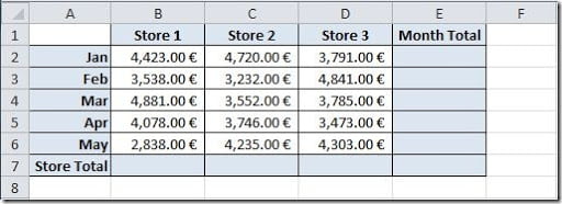
Excel has an AutoSum feature that can save us lots of time when we are working with data tables. Let’s see a practical example. We have a monthly store sales table, like this:

Now we want to put monthly total sales and a stores year to date total sales. For the monthly sales total, we could put a formula =SUM(B2:D2) on cell E2 and copy down. For the stores year to date total sales, we could put, on cell B7, a formula =SUM(B2:B7) and copy to the right. But all of this can be done using Excel’s AutoSum feature. This feature is so popular that Microsoft putted in two different locations of our menu bar. It can be found on the Home tab, on the Editing group (right side of the menu bar):

and it can be found on the Formulas tab, on the Function Library:

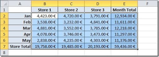
To use this feature on our table, and put all of the totals mentioned before, on one single step, we need to select the range of cells with the values and, here’s the trick, we need to select one more empty row of cells (for the stores year to date total sales) and one more empty column of cells (for the monthly total sales). In this example, we need to select the B2:E7 range of cells. After that, let’s click on one of the AutoSum buttons mentioned before. The result will be like this:

Now we have all of the totals that we wanted. To make this operation even easier to do, instead of clicking on one of the menu buttons, we can use the shortcut keys Alt+= (press Alt key and then the Shift and the key with the = symbol). The result will be exactly the same.

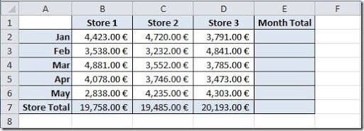
This AutoSum feature can be use to put totals in other ways. For example, if we select only the range of cells with the values (no empty rows or columns), in this case if we select cells B2:D6, and we click on the AutoSum button, we will get only the column totals, placed beneath the first available row below our data, in this case, on row 7. The result will be like this:

This AutoSum button can be used, instead of sum’s, for other functions like average, count number, etc. You can check the available options clicking on the little arrow on the lower part of the AutoSum button:

As you can see, the feature is very useful, and very easy to use. It will certainly save you lots of time, when working with data tables.

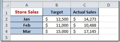
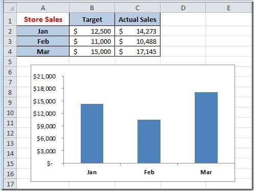
I’ve a table of data with target values and actual values, by month, like this:

I want to create a bar chart with this data, something like this:

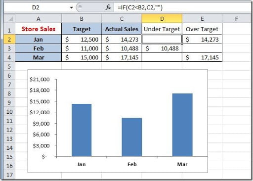
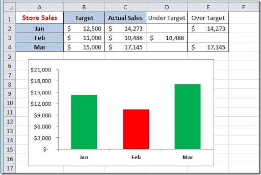
But I would like, for better understand the data, to see if the actual values, for each month, are above or below the target value. If it’s on target, or over the target, I would like the month bar to show up in green color and, if it’s below target, to show up in red color. This can be done by adding two columns to our table, one for the results “under target” and one for the results “over target”. On this two columns, what we are doing, is to check if the actual sales value is less that the target, then show the actual value; if not, leave the cell blank. This for the “under target” column. For the “over target” column, we are going to check if the actual sales value is equal, or greater than the target value. If true, then, show the actual sales value; if not, leave the cell blank. The result will be like this:

For the “under target” column, put this formula on cell D2 and copy down:

=IF(C2<B2,C2,””)

For the “over target” column, put this formula on cell D2 and copy down:

=IF(C2>=B2,C2,"")

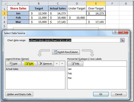
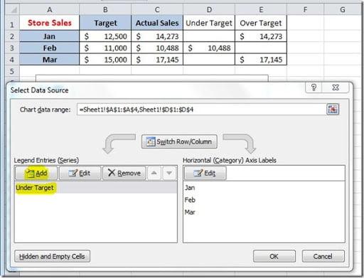
Now we need to change our chart data source. If you right click on your chart and select “Select Data”, it will open the “Select Data Source” dialog box, like this:

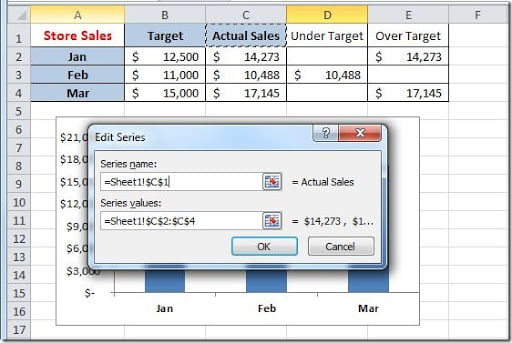
As you can see, your chart has only one data series. We are going to work with two data series: one for the “under target” values and one for the “over target” values. To start, we are going to change the series values for the existing series. For that, click on the Edit button on the Series box, on the left of the dialog box. This is pointing to column C, as you can see on the image below. We need to change the “Series name” to “=Sheet1!$D$1” and the “Series values” to “=Sheet1!$D$2:D$4” and click the OK button.

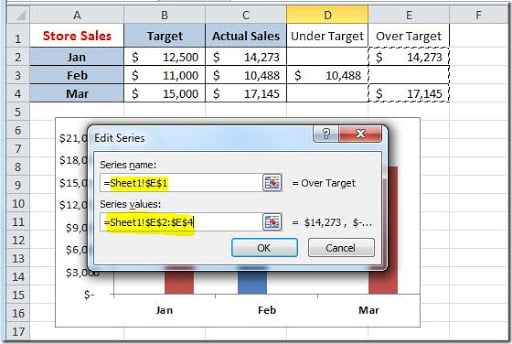
Our chart series in now point it out to the “under target” column. We need to add the second series for the “over target” values. Click on the Add button, on the Series box:

Fill out the “Edit Series” dialog box, like this, and click on the OK button:

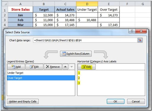
As you can see, you need to specify the “Horizontal Axis Labels” for this new series because it’s not showing up the months names. Just click on the Edit button and select the “=Sheet1!$A$2:$A$4” range.

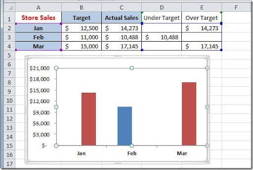
Close the “Select Data Source” dialog button, by clicking the OK button, and your chart should now look like this:

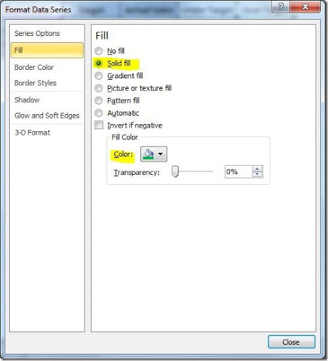
We need to change the color of our series bars to display the “under target” values as red bars and the “over target” values as green bars. Just right click on the “over target” bars and select “Format Data Series”. Go to the Fill group and select “Solid fill” with a green Fill Color. Click the Close button when finished.

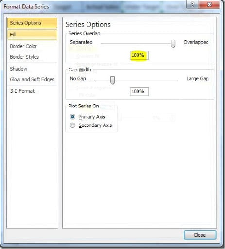
Do the same for the “under target” series but for this select a red Fill Color. Before clicking on the Close button, select the “Series Options” group and on the “Series Overlap”, put 100% so that the chart bars appear center between each month.

When you click the Close button, the result should be like this:

Try changing any value on the B2:C4 range to see the conditional formatting of the chart adjust the colors.

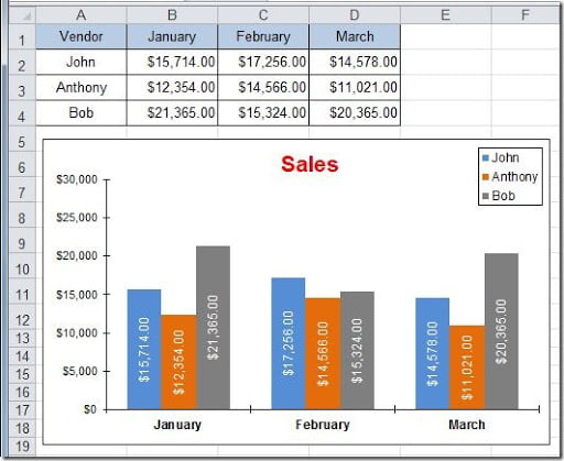
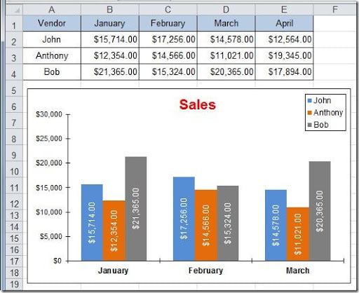
This is a common task on Excel. We have a chart and we need to update the data displayed by adding more data. For instance, we have a chart that displays data from January to March and we need to add data for a new month. Let’s see how we can do this. We have this existing chart:

Now lets add a new column to our table to add the April sales data, like this:

There are several ways of adding and additional column of data to our chart. Let’s see some:

Method 1: This is the easiest way of doing this but it’s now always possible to to. Instead of putting the new data on the right side of the last column, insert a new column between columns C and D, copy the March data into this new column and put the April values on column E. Because you are adding a new column inside the source data range of the chart, Excel will adjust to accommodate this new column. As I said, this is not always possible if you have more data below this table. If you insert a new column, it will mess the data below.

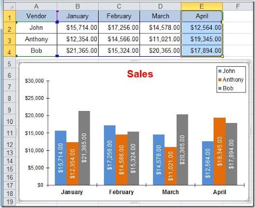
Method 2: Put the April data on column E. Select cells E1:E4 and press Ctrl+C (Copy). Then click on the chart to select it and press Ctrl+V (Paste). You will have your new data displayed on the chart, like this:

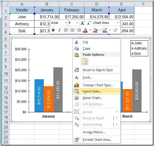
Method 3: This is the usually method that most people use. Right click on the chart and select the Select Data option, of go to the Design tab and on the Data group, click on the Select Data button.

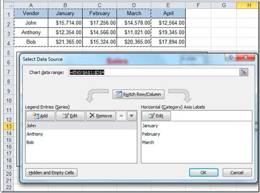
A Select Data Source dialog box opens and the chart source range get’s highlighted with the “marching ants”.

With the cursor on the “Chart data range” field, just select the new data range, in this case select A1:E4. Click the OK button and your chart will be updated with the new data.

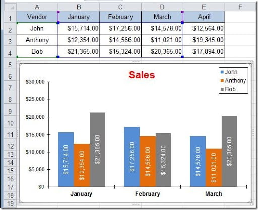
Method 4: Click on the chart. If you look at your table now, you can see blue, green and violet lines around the cells.

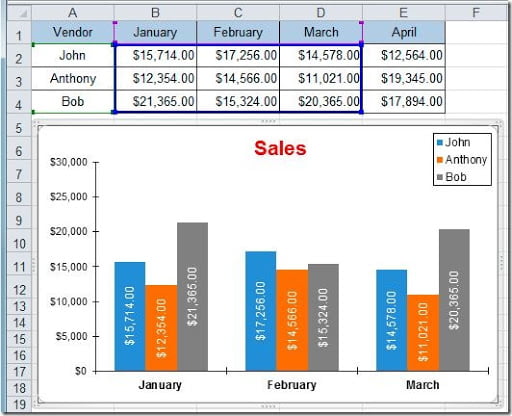
If you pass the mouse on top of the blue line, it will get thicker showing you the actual source data of your chart, like this:

Just drag the line, pushing from one of the blue squares on the corners, so that you get the new range of data selected, in this case range B2:E4 and release the mouse button so that your chart gets updated.

As you can see, there are many ways of doing the same thing in Excel. You just need to choose the one that you like it more.

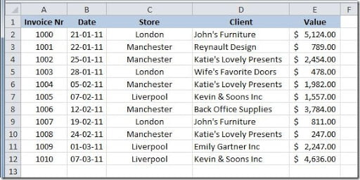
This is a very handy trick. We have a table, like this:

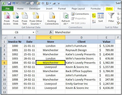
We now want to get the subtotals of the Value column, for each Store. First thing that we need to do, is to sort the table by the Store column. The easiest way is to click on any cell on the column (in this case, C2:C12), go to your Data tab and click on the “Sort A to Z” button, like this:

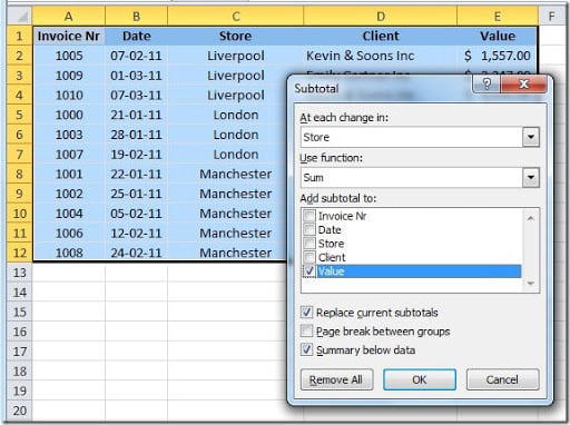
We now have our table sorted by the Store column. To add the subtotals, on your Data tab, you’ll find a Subtotal button, on your Outline group. Click it and a Subtotal dialog box will open, like this:

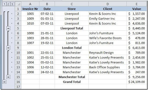
Now you can choose what is the column that you want to group (“At each change in”), in this case is the Store column, what is the function you want to use, we want to Sum, and what is the column that you want to sum, that is the Value column. Just click OK and your sheet will now look like this:

As you can see, you now have an Outline column to the left of your sheet and a subtotal for each Store and a Grand Total in the end. Let’s see what you can do with this new Outline columns. Click on the “1” button, on the top of the Outline column and you will hide all of the details on your table, leaving you only with the Grand Total, like this:

If you click on the “2” button, you will get only the subtotals by store and the Grand Total, like this:

If you click on the “3” button, you will get your complete table again. You can always click the “+” and “-“ buttons to expand or collapse some of your groups. If you want to remove your subtotals, and go back to your original table, just select a cell on your table, go to the Data tab, click the Subtotal button again and on the dialog box that opens, click on the “Remove All” button.

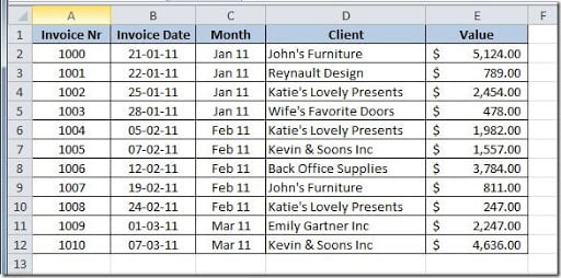
You have a table of data and you hide some rows and columns and you want to copy only the visible cells into another sheet? I’m going to show you some techniques that you can use to do that. Let’s see how our original table looks like:

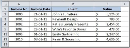
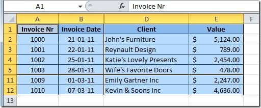
Now, let’s hide some rows and columns so that our table looks like this:

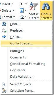
If you select the entire table (cells A1:E12) and just copy and paste (Ctrl+C and Ctrl+V) it into another sheet, it would copy all rows and columns and would look like the original table. That’s not what we want to do, we just want to make a copy and show only the 7 rows and 4 columns that we see on the image above. For that we need to select the visible cells only so that we can copy only those. Let’s select again cells A1:E12 but this time we’re going to select first only the visible cells, before copying. We can do this by just using the shortcut Alt+; (semicolon) or you can go to the Home menu bar, on the Editing group, and click on the Find & Select button and choose Go To Special option.

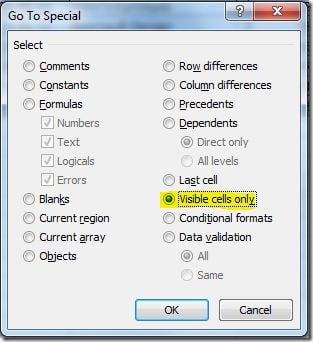
Instead of going to the menu bar, you can just press F5 or Ctrl+G to open the “Go To” dialog box and then just press the Special button on the bottom. On the Go To Special dialog box, select the “Visible cells only” option:

This will select only the visible cells, as you can see on this image:

Now you can just Ctrl+C (Copy) and Ctrl+V (Paste) it into another location. This will only copy the visible cells, like you wanted.
If you are working with Filters, you don’t need to use this techniques because, when you copy filtered data, it only copies the visible cells already.

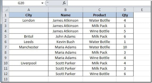
This is a common need for Excel users. Let’s imagine that you have a table, like this:

As you can see, only the first record, for each city, is filled on column A. If you needed to sort this table, you would loose the information of the City on the rows where column A is not filled. So, you need to fill the blanks on column A.

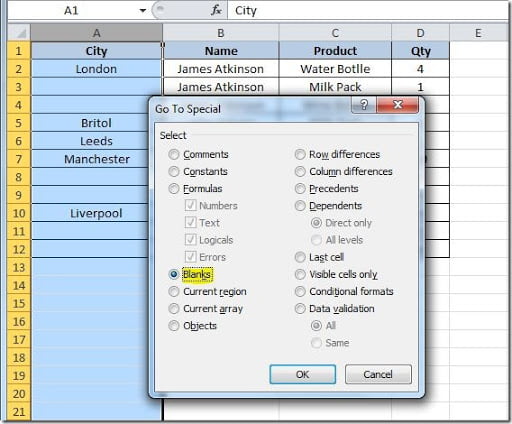
To start, let’s click on column A header to select this column. Then press F5 or Ctrl+G to open the “Go to” dialog window. Here, click on the “Special…” button and, on the dialog window that opens, select “Blanks” option, like this:

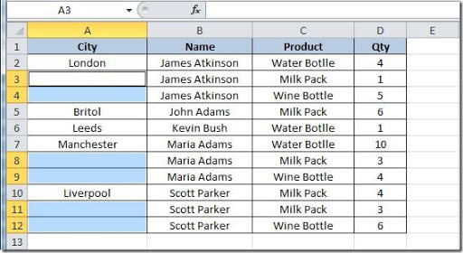
Click the OK button and you will have only the blank cells of column A selected, like this:

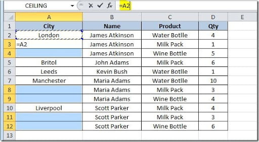
Now, on your formula bar, write “=” and press the first filled cell on column A, in this case, cell A2, like this:

As you can see, the formula that you’ve entered on the formula bar, is being written on cell A3, because it’s the first cell on the ones that are selected. Now, instead of pressing just Enter, press Ctrl key and then Enter (holding the Ctrl key) to insert this formula in all of the selected cells. The result will be like this:

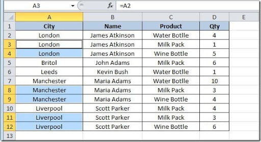
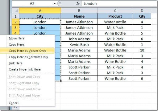
You now have all of your blank cells on column A filled with the value from the first filled cell above. Now you need to convert the formulas to text. For that, just select the cells on your column A, in this case range A2:A12. Click on the edge of the selection range with your right mouse button and drag it slightly to the column to the right and then back to column A and release the right mouse button. A new option menu will appear, like this:

Select the “Copy Here as Values Only” option and your formulas will be replaced by the cell values. Now you can use your data table is ready to be used on sorts.