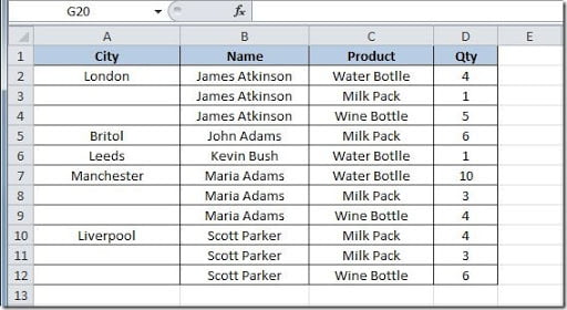
This is a common need for Excel users. Let’s imagine that you have a table, like this:
As you can see, only the first record, for each city, is filled on column A. If you needed to sort this table, you would loose the information of the City on the rows where column A is not filled. So, you need to fill the blanks on column A.
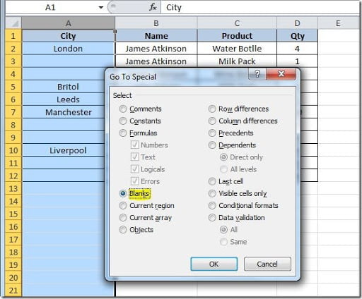
To start, let’s click on column A header to select this column. Then press F5 or Ctrl+G to open the “Go to” dialog window. Here, click on the “Special…” button and, on the dialog window that opens, select “Blanks” option, like this:
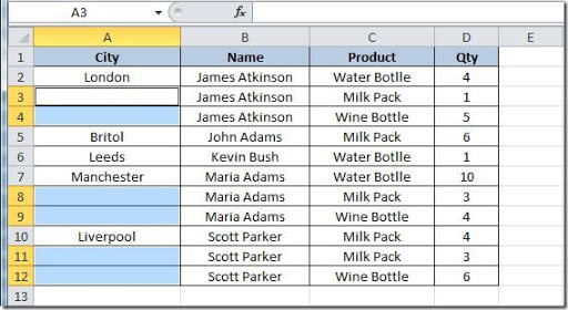
Click the OK button and you will have only the blank cells of column A selected, like this:
https://travelrouteplanner.com/vacation/how-many-days-is-summer-vacation/.
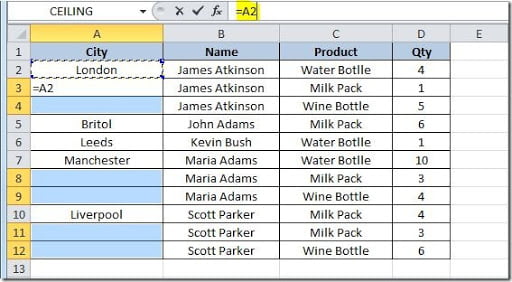
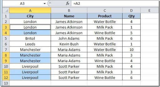
Now, on your formula bar, write “=” and press the first filled cell on column A, in this case, cell A2, like this:
As you can see, the formula that you’ve entered on the formula bar, is being written on cell A3, because it’s the first cell on the ones that are selected. Now, instead of pressing just Enter, press Ctrl key and then Enter (holding the Ctrl key) to insert this formula in all of the selected cells. The result will be like this:
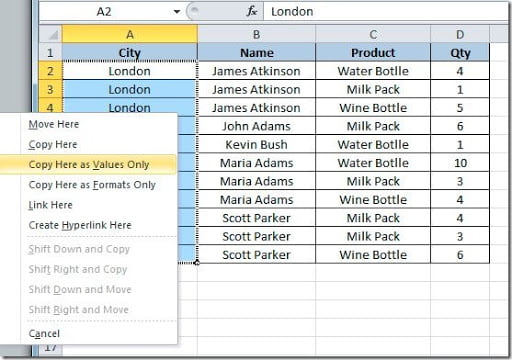
You now have all of your blank cells on column A filled with the value from the first filled cell above. Now you need to convert the formulas to text. For that, just select the cells on your column A, in this case range A2:A12. Click on the edge of the selection range with your right mouse button and drag it slightly to the column to the right and then back to column A and release the right mouse button. A new option menu will appear, like this:
Select the “Copy Here as Values Only” option and your formulas will be replaced by the cell values. Now you can use your data table is ready to be used on sorts.
