Excel has a function to locate a value on a range of cells and return the number of the row where the value is found, it’s the MATCH() function. The syntax is like this:
MATCH(lookup_value,lookup_array,match_type)
lookup_value is the value that we want to look for and lookup_array is the range of cells where we want to search. match_type can have 3 values:
1 - finds the largest value that is less than or equal to lookup_value. Lookup_array must be placed in ascending order;
0 - finds the first value that is exactly equal to lookup_value
-1 - finds the smallest value that is greater than or equal to lookup_value. Lookup_array must be placed in descending order.
If match_type is omitted, it will assume to be 1.
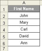
Here’s an example. We have the following table:

We want to find the name Mary on the range of A2:A6. So we should use this formula:
=MATCH("Mary",A2:A6,0)
This will return 2 because the name Mary can be found on cell A2.
