This article was originally written for the Microsoft Excel Blog. The purpose of this article is to show Excel users some technique’s, and Excel functions, that they can use to lookup up a value on a table, using more than one criteria. If you have only one criteria, it’s simple, you can use a plain VLOOKUP formula to do that. If you want to use more than one, then there are lots of ways of doing it, using several of Excel’s functions like VLOOKUP, LOOKUP, MATCH, INDEX, etc.
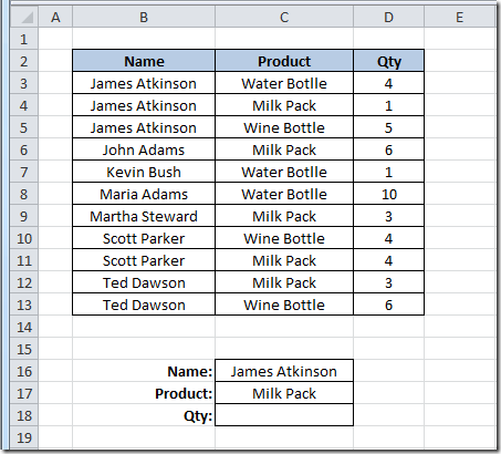
Let’s see a scenario where we want to use two criteria’s to return a value from a table. This is the data table that we have:
As you can see, we want to use a “Name” and “Product” criteria to return a “Qty” value on cell C18. We are going to look for the Name “James Atkinson” and the Product “Milk Pack” to return the Qty from the table. Because the value that we want to return is a number, we can use a simple SUMPRODUCT() formula in C18 cell, like this:
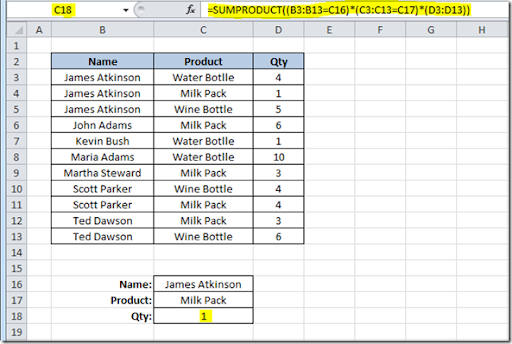
=SUMPRODUCT((B3:B13=C16)*(C3:C13=C17)*(D3:D13))
What this does is look on the range B3:B13 for the value on cell C16 and on the range C3:C13 for the value on cell C17 and where it finds both, return the value on column D, from the same row where it found both criteria’s. Here’s how it will look:
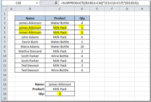
It is returning the value 1 that corresponds to the value on cell D4 because it found “James Atkinson” Name on row 4 and also “Milk Pack” on the same row, thus returning the value of column D from that row. Let’s just change value on cell C5 from “Wine Bottle” to “Milk Pack” to see what happens with the formula on cell C18:
Because our formula found two lines where both criteria’s were found, it is summing the values on column D on rows where they were found, giving us a Qty of 6.
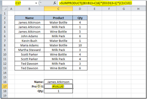
This technique cannot be used is we wanted to look for two criteria’s and return a text result. For instance, this, would not work:
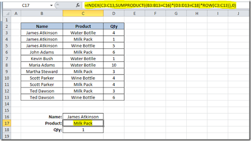
We are looking for the Name “James Atkinson”, where the Qty is 1 and we want to return the Product name that matches this two criteria’s. This formula would give us a #VALUE error! Instead we could use a formula using a combination of SUMPRODUCT, INDEX and ROW functions, like this:
=INDEX(C3:C13,SUMPRODUCT((B3:B13=C16)*(D3:D13=C18)*ROW(C3:C13)),0)
We use the SUMPRODUCT function to find out the row where both criteria’s are found and return the corresponding row number using the ROW function. Then we use it on the INDEX function to return the value on the array C3:C13 that is on the row number provided. The result will be like this:
This could also be done using a different technique. You could use this formula on cell C17:
=LOOKUP(2,1/(B3:B13=C16)/(D3:D13=C18),(C3:C13))
The result will be the same as the previous solution. What this formula does, is divide 1 by an array of True/False values (B3:B13=C16) and then by another array of True/False (D3:D13=C18). This will return 1 or a #DIV/0 error. Using 2 as the lookup value, then the match will be with the last numeric value in the range, i.e. the last row where both conditions are True. This will be our "vector form" of the LOOKUP, so then you get the corresponding value returned from C3:C13. I used 2 as the LOOKUP value but it can be any number, starting at 1. If the formulas don’t find any match, of course you will get a #N/A error!
You could also use an array formula, using the MATCH function, like this:
{=INDEX(C3:C13,MATCH(1,(B3:B13=C16)*(D3:D13=C18),0))}
On this technique, I used the MATCH function to find the row where both conditions are found. This will return a value of 1 that will be matched to the 1 that was used as the lookup value of the MATCH function, thus returning us the row where the conditions are met. Using the INDEX value, we look for the value that is on the range C3:C13, that is on the row that was returned from the MATCH function, in this case, it was row 2, that corresponds to the second row on C3:C13.
All of this examples show you how to use two criteria’s for your lookups. It’s easy to do it if you have more than two, just add then to your formulas. Here how the formulas presented before, would look if you add one more criteria:
=SUMPRODUCT((B3:B13=C16)*(C3:C13=C17)*(E3:E13=C18)*(D3:D13))
=INDEX(C3:C13,SUMPRODUCT((B3:B13=C16)*(D3:D13=C18)*(E3:E13=C18)*ROW(C3:C13)),0)
=LOOKUP(2,1/(B3:B13=C16)/(D3:D13=C18)/(E3:E13=C18),(C3:C13))
{=INDEX(C3:C13,MATCH(1,(B3:B13=C16)*(D3:D13=C18)*(E3:E13=C18),0))}
As you can see, depending on your data tables, you can use several different techniques to lookup your values, using different Excel functions. Hope that you can apply this to your own Excel sheets.
