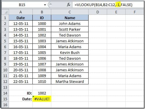
VLOOKUP() function only returns values from the columns to the left of the key field. You can’t build the formula and give it a column index number of –1, for instance. This is will result on a #VALUE error, like on the following example:
Find entertainment daily at goojara movie channel.
On this example, we want to retrieve the value on the Date column that matches with the ID on cell B14 so we putted a –1 column index number on the function that didn’t worked.
A simple way of going around this problem is to build our own VLOOKUPNEG (as from negative) function that works with negative column index numbers and can return values to the left of the key field, in this case, the Date value that is on the left of the ID column. So, this is the UDF (User Defined Function) that you can create:
Function VLOOKUPNEG(lookup_value, table_array As Range, col_index_num As Integer, CloseMatch As Boolean)
Dim RowNr As Long
RowNr = Application.WorksheetFunction.Match(lookup_value, table_array.Resize(, 1), CloseMatch)
VLOOKUPNEG = table_array(RowNr, 1).Offset(0, col_index_num)
End Function
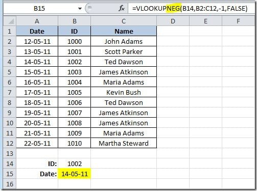
Using this UDF, on the same example, we will get this result:
Now, on cell B15, we are already getting the Date that matches the 1002 ID that was on cell B14: 14-05-11!


