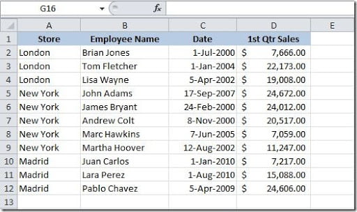
This is just a simple trick that can help you improve your tables printing. Imagine that you have a table like this below:
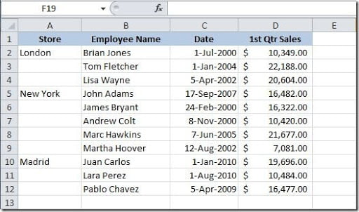
Many people prefer not to print the tables with the same stores location repeated on column A, for each line. Many would prefer to print the table looking like this:
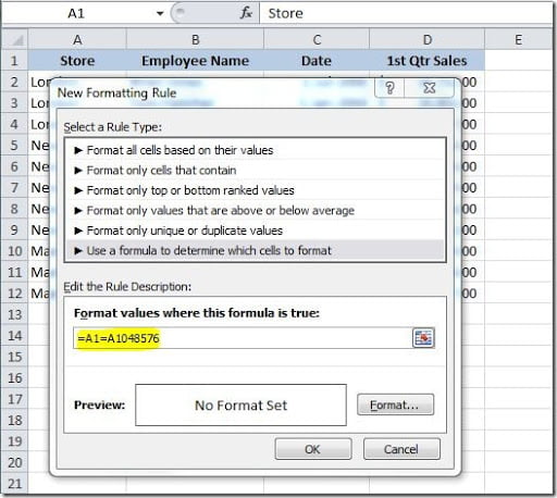
To achieve this, just click on column A, to select the entire column, and then, on the Home menu tab, click on the Conditional Formatting button and then on New Rule option. Then, on the dialog box that opens up, on the “Select a Rule Type” field, choose the last one “Use a formula to determine which cells to format”. Now, on the “Format values where this formula is true” field, we will enter =A1=A1048576, like this:
This will tell Excel that if any value on column A is equal to the value above, then this formula is true. We use 1048576 because it’s the number of rows that Excel 2010 has, has you can see here. Then we need to set the format to apply when the formula is true. Because we want to hide the cell content, in this case we will use a white font color, so click on the Format button and, on the Font tab, on the Color field, choose the white color. Click OK button twice to finish. Your table will look like the second example that I showed here.
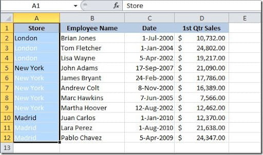
The values on column A are still there, in each row, but they don’t show up on the printing. If you select column A, you can see that all of them are still there, as you can see on this image:
The advantage of keeping the values is that, if you need to do a sort on your data table, you can do it without loosing the correlation between the rest of the columns with column A. As you can see, this is a very small table, it’s easy to do this for each store location but if we were talking of a table with thousands of rows, this trick will save you lots of time.


