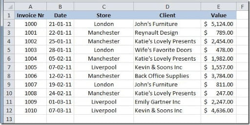
This is a very handy trick. We have a table, like this:
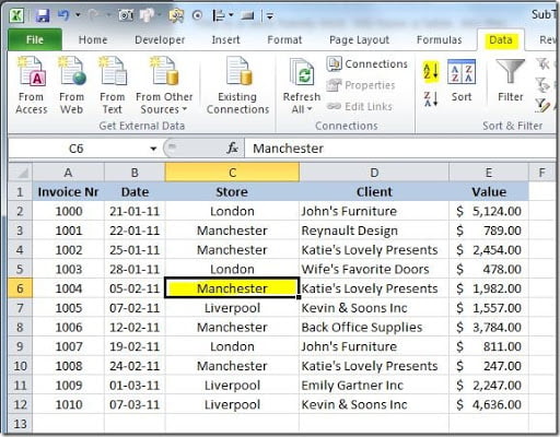
We now want to get the subtotals of the Value column, for each Store. First thing that we need to do, is to sort the table by the Store column. The easiest way is to click on any cell on the column (in this case, C2:C12), go to your Data tab and click on the “Sort A to Z” button, like this:
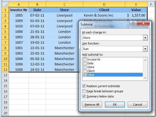
We now have our table sorted by the Store column. To add the subtotals, on your Data tab, you’ll find a Subtotal button, on your Outline group. Click it and a Subtotal dialog box will open, like this:
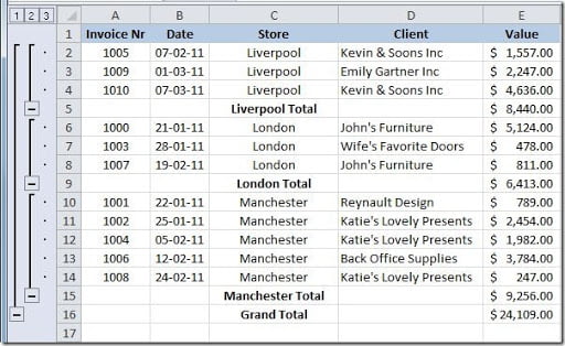
Now you can choose what is the column that you want to group (“At each change in”), in this case is the Store column, what is the function you want to use, we want to Sum, and what is the column that you want to sum, that is the Value column. Just click OK and your sheet will now look like this:
As you can see, you now have an Outline column to the left of your sheet and a subtotal for each Store and a Grand Total in the end. Let’s see what you can do with this new Outline columns. Click on the “1” button, on the top of the Outline column and you will hide all of the details on your table, leaving you only with the Grand Total, like this:
If you click on the “2” button, you will get only the subtotals by store and the Grand Total, like this:
If you click on the “3” button, you will get your complete table again. You can always click the “+” and “-“ buttons to expand or collapse some of your groups. If you want to remove your subtotals, and go back to your original table, just select a cell on your table, go to the Data tab, click the Subtotal button again and on the dialog box that opens, click on the “Remove All” button.


