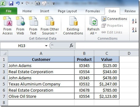
In previous versions of Excel, removing or highlighting duplicates was not a natural thing of Excel, you would need some tricks to do it. Excel 2010 now provides a tool to handle this easily. Take a look at this sample data:

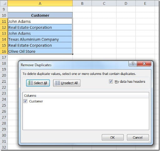
As you can see, there are some Customers and Products duplicated on our table. We want to get a list of unique customers. For that we need to copy the data from column A to another section of our worksheet (in this case the range A1:A7). Then select a single cell within the data set. Go to your menu bar and on the Data tab click on the Remove Duplicates button. A Remove Duplicates dialog box will open like this:

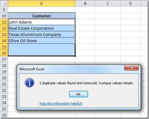
Excel will assume that you have headers on your data and will check the “My data has headers” check box and the name of your columns will appear on the list below. Here is where you will select the fields that you want to make unique records. In this case it’s just the Customer field. Click OK to close the dialog box and you will get a message with the number of duplicates found and remove and the number of unique records that remained.

In this example we used just a single column to check for duplicates but we could check for duplicates using more fields. We could check for unique combination of Customers and Product. For that, on the Remove Duplicates dialog box, just select both columns from the list.
Instead of removing your duplicate records, you may want to just highlight them on your sheet so that you can see witch are duplicated. You can do that by using Conditional Formatting option under Home tab. Please check the Highlight Duplicates article for that.
Showing posts with label Duplicates. Show all posts
Showing posts with label Duplicates. Show all posts
