Excel-User.com

This function returns a value corresponding to the type of Excel error. This is the syntax:

ERROR.TYPE(error_val)

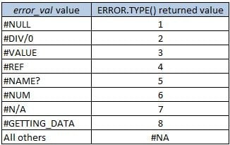
error_val is a reference to a cell that has a formula that you want to check if it returns an error value. Here are the possible return values:

This function can be very useful to check if a certain formula returns an error, so that you can display a custom error message to the user. For that you can use the IF() function combined with the CHOOSE() function, like this:

=IF(ERROR.TYPE(A2)<=8,CHOOSE(ERROR.TYPE(A2),"Ranges not intersecting","0 Divisor","Wrong data type","Invalid cell reference", "Unrecognized range or function name","Number error","Inappropriate function argument","Waiting for query data"),"")

This formula will check if there is an error on cell A2 formula and if it returns a ERROR.TYPE value will choose the appropriate error message to display on the cell where this formula is placed. If there is no error, it will return nothing. Here are some examples of the use of it:

You can improve this formula to give you the cell address where you have the error by using the CELL() function, like this:

=IF(ERROR.TYPE(A3)<=8,CHOOSE(ERROR.TYPE(A3),"Ranges not intersecting","0 Divisor","Wrong data type","Invalid cell reference", "Unrecognized range or function name","Number error","Inappropriate function argument","Waiting for query data")& " on cell " & CELL("address",A3),"")

This will return a message like this instead:

Hope this is useful to get your worksheets more user friendly.

Maybe you already had the needs to extract the first and last name from a string containing the complete name of a customer. I know I did! This is a good example of the application of this article.
To get the first word from a string, we need to find the first space on the string. For that we can use the FIND() function. This function works from left to right so is perfect for finding the first space on the string. Then we want to retrieve the word to the left of the fist space. For that we will use the LEFT() function. Here’s how we can build our formula:

=LEFT(A2,FIND(" ",A2)-1)

Because we can be dealing with different strings and some may not have a space, we need to check for errors on our formula so we should use the IFERROR() function on Excel 2007 and 2010 like this:

=IFERROR(LEFT(A2,FIND(" ",A2)-1),"")

This way, if we find any error on our formula, instead of showing #VALUE on the cell, we just leave it blank when this happens. In previous versions of Excel the IFERROR() function doesn’t exists so we need to use the ISERR() function that is compatible with all Excel versions. Our formula needs to change to this:

=IF(ISERR(FIND(" ",A2)),"",LEFT(A2,FIND(" ",A2)-1))

To get the last word from a string is not so easy because what I’ve mentioned earlier, the FIND() function works from left to right so we need to find the last space on the string and get the text to the right of it. Here’s the formula:

=RIGHT(A2,LEN(A2)-FIND("*",SUBSTITUTE(A2," ","*",LEN(A2)-LEN(SUBSTITUTE(A2," ","")))))

As in the previous formula, we need to check for errors on our formula to avoid the #VALUE error message, so our formula turns to this:

=IFERROR(RIGHT(A2,LEN(A2)-FIND("*",SUBSTITUTE(A2," ","*",LEN(A2)-LEN(SUBSTITUTE(A2," ",""))))),A2)

To have a formula that is compatible to all Excel versions, we need to change our formula to this:

=IF(ISERR(FIND(" ",A2)),"",RIGHT(A2,LEN(A2)-FIND("*",SUBSTITUTE(A2," ","*",LEN(A2)-LEN(SUBSTITUTE(A2," ",""))))))

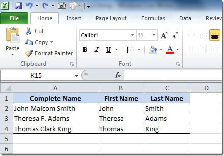
This will produce something like this example:

The IF() function is one of the most used in Excel. It’s very simple to use. The syntax for this function is:

IF(logical_test,value_if_true,value_if_false)

logical_test is the value or expression that we want to evaluate. value_if_true is the result if the condition of logical_test is true and value_if_false is the result if the condition is false.

Examples:

=IF(A2=100,"True","False") will check if there is a value 100 in cell A2. If true, will put on the cell where we have the formula, the value “True”. If the value in cell A2 it’s not 100 the formula will return “False” on the cell.

=IF(AND(A2=100,A3=200),"True","False") this is the same as the last example with the exception that in this case we are checking two condition and only if both are true, the result will be “True”.

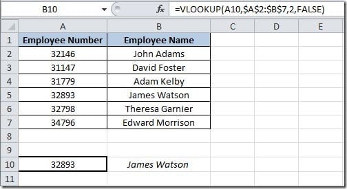
If we have a table of data, like the one shown bellow, and based on a value of that table want to return the value from another column we can use the VLOOKUP() function.

 
The syntax for this function is:

VLOOKUP(lookup_value,table_array,col_index_num,range_lookup)

In our example, on cell B10 I've putted this formula:

=VLOOKUP(A10,$A$2:$B$7,2,FALSE)

First we have the lookup value that is the value that we want to check is it's on the table. In this example is the value on cell A10.

Then we have the table array. This is the range of cells where we want to check for the value on cell A10. In this case, we want to lookup the value on range A2:B7. If it finds the value of A10, it will the return the value referred by the col_index_num argument of the function. In this case we want to return the value from column 2 (the employee name).

The range_lookup argument is optional and it can have TRUE or FALSE value. If you put TRUE or omit this argument, it will return an approximated match. If it doesn't find the value of the lookup_value it will return the next largest value that is less than the lookup_value. If you put FALSE, it will find an exact match and if it doesn't find one it will return the error value #N/A.

So, on this example, we want to find the value 32893 and get the corresponding value from column 2, in this case the returned value will be James Watson.

If the value specified on the lookup_value is not found, and the range_lookup is FALSE, then the formula will return a #N/A error value. We can change our formula so that it doesn't display this error with this formula:

=IF(ISNA(VLOOKUP(A10,$A$2:$B$7,2,FALSE)),"",VLOOKUP(A10,$A$2:$B$7,2,FALSE))

In this case we use two more functions, the IF and ISNA. I will not explain the IF function in this article, will handle this function on a separated article on the future.

The ISNA() function checks if the VLOOKUP() function returns a #N/A error value. So this formula will check if the VLOOKUP() function returns #N/A. If it does, the cell will be empty. If it doesn't it will show the result of the VLOOKUP function.