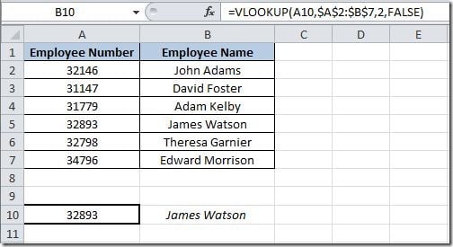
If we have a table of data, like the one shown bellow, and based on a value of that table want to return the value from another column we can use the VLOOKUP() function.

The syntax for this function is:
VLOOKUP(lookup_value,table_array,col_index_num,range_lookup)
In our example, on cell B10 I've putted this formula:
=VLOOKUP(A10,$A$2:$B$7,2,FALSE)
First we have the lookup value that is the value that we want to check is it's on the table. In this example is the value on cell A10.
Then we have the table array. This is the range of cells where we want to check for the value on cell A10. In this case, we want to lookup the value on range A2:B7. If it finds the value of A10, it will the return the value referred by the col_index_num argument of the function. In this case we want to return the value from column 2 (the employee name).
The range_lookup argument is optional and it can have TRUE or FALSE value. If you put TRUE or omit this argument, it will return an approximated match. If it doesn't find the value of the lookup_value it will return the next largest value that is less than the lookup_value. If you put FALSE, it will find an exact match and if it doesn't find one it will return the error value #N/A.
So, on this example, we want to find the value 32893 and get the corresponding value from column 2, in this case the returned value will be James Watson.
If the value specified on the lookup_value is not found, and the range_lookup is FALSE, then the formula will return a #N/A error value. We can change our formula so that it doesn't display this error with this formula:
=IF(ISNA(VLOOKUP(A10,$A$2:$B$7,2,FALSE)),"",VLOOKUP(A10,$A$2:$B$7,2,FALSE))
In this case we use two more functions, the IF and ISNA. I will not explain the IF function in this article, will handle this function on a separated article on the future.
The ISNA() function checks if the VLOOKUP() function returns a #N/A error value. So this formula will check if the VLOOKUP() function returns #N/A. If it does, the cell will be empty. If it doesn't it will show the result of the VLOOKUP function.
