 It will look something like this:
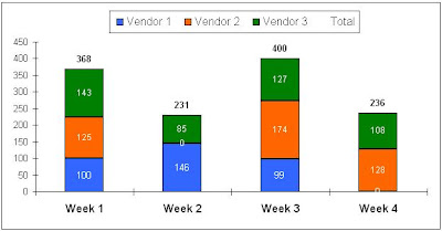 As you can see, the chart will display the zero values. If you want to hide the zeros, you have two ways of doing:
Method 1:
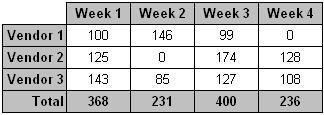
1) Select the range of cells where you have the values for your chart
2) Right click and select Format Cells
3) On the Number tab, on Category, select Custom
4) In the "Type" box you will see the current format for the range you selected
5) Put the cursor on the end of the content of the Type box and enter 0,0;;; it it will look something like this picture:
 6) Your zero values will be hiden now
 Method 2:
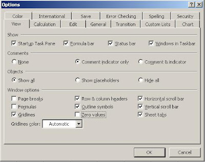
Go to Tools, Options and on the View tab, under Window option, uncheck the Zero values options, like this: