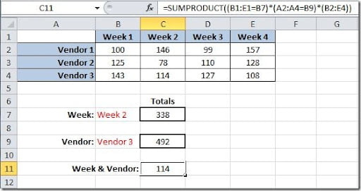
Sometimes we want to sum values from a table based on conditions that we input into another cell. Take a look at the table below. Here we have a table of weekly values for each vendor.

In this case we want to input on cell B7 the week value and get the total for this week on cell C7. This can be done using the SUMPRODUCT() function. The syntax for this function is like this:
SUMPRODUCT(array1,array2,…) you can have up to 30 arrays.
The formula in C7 for this will:
=SUMPRODUCT((B1:E1=B7)*(B2:E4))
Checks on range B1:E1 for the value in cell B7 and sums the values under that value. On this example the value "Week 2" can be found on C1 so the sum will be done with the values from C2:C4 and the result will be 338.
Another example is putting in B9 the vendor name and get the total for this vendor on cell C9. The formula will be like this:
=SUMPRODUCT((A2:A4=B9)*(B2:E4))
Checks on range A2:A4 for the value in cell B9 and sums the values for that row where it finds the vendor. On this example the vendor "Vendor 3" can be found on row 4 so the sum will be done with the range B4:E4 and the result will be 492.
Finally we want to get the value for Week 2 for Vendor 3. We can use also the SUMPRODUCT function like this:
=SUMPRODUCT((B1:E1=B7)*(A2:A4=B9)*(B2:E4))
It will return the value 114 that corresponds to Vendor 3 (row 4) and Week 2 (column C).
These are simple examples of how you can use the SUMPRODUCT function. It can be used in more complex formulas that I will address later on another article.
