This is a real situation that many of us already experienced! We have a list of data and we need to get the top N values from that list. Of course we can sort descending the list and get the top values, but many times we can’t sort the source data (it may be used on another report, for instance). We can use the LARGE() function to get the nth largest value from a range of values. The syntax is like this:
LARGE(array, k)
array is the range of data from where we want to get our top values
k is the position on the range of data to return
k is the position on the range of data to return
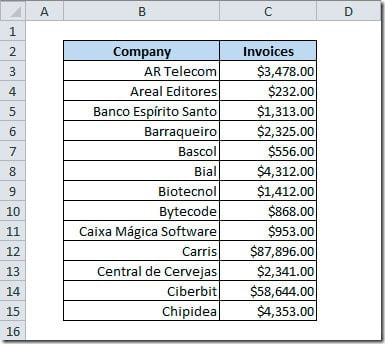
So, let’s see an example on how to apply this function to get our top values. Our source data is like this:
In this example we want to get the Top 5 companies by Invoices value. We will be putting the values on cells B17:C21.
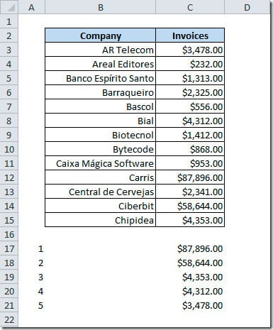
To start, let’s put the numbers 1 to 5 on cells A17:A21. Now, on cell C17 let’s put our formula, like this:
=LARGE($C$3:$C$15, A17)We will be looking on cells C3:C15, where we have our Invoices values, for the first largest value, that why we are using cell A17 that has the number 1 on it. Use the dollar signs on the array argument so that when we copy the formula to the next rows it will keep the reference to our Invoices values that are on C3:C15. Now copy the formula on cell C17 to the rest of the cells (C18:C21). This is how our sheet should look like:
So, now we have the top 5 Invoices values but wee need to fill the companies names. For that we will use the MATCH() function to get the row number within range C3:C15 that has the value that matches C17. The MATCH formula will be like this:
=MATCH(C17,$C$3:$C$15,0)
For the value in C17, this formula would return 10 because the value on this cell is coming from row 10 of our range source. This is not row 10 of our sheet but row 10 of our source! Now with this information we can get the company name that is on this row. For that we will use the INDEX() function like this:
=INDEX($B$3:$ B$15,10)
This would get the company’s name on row 10 of our source data.
Combining both formulas, it will look like this:
=INDEX($B$3:$B$15,MATCH(C17,$C$3:$C$15,0))
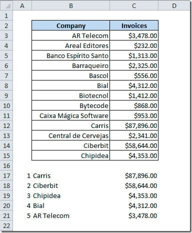
Put this formula on cell B17 and copy to the other cells on B18:B21.
The result will be like this, where we get on cells B17:C21 the top 5 values of Invoices from our source data on B3:C15:
Hope that this article can be useful for your work.


