Excel has a powerful pack of financial functions that you can use. Most of them are only used by people with specific needs, but some can be useful for the majority of people to make calculations on loans for instance. One of the most useful functions is PMT(). It can be used to calculate the monthly payment on a loan. Here’s the syntax:
PMT(rate, nper, pv, fv, type)
rate is the interest rate for the loan
nper is the number of payments for the loan
pv is the present value, is the loan amount
fv is an optional value. It can be the final payment for the loan. If omitted, it will assume 0
type can be either 0 or 1. It indicates when the payments are due. Default value is 0 assuming that the first payment is due after a month or you can set this to 1 if the first payment is to be done when the loan is issued.
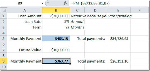
Let see a practical example how we can use this function to calculate the monthly payment on a $30,000 loan, with 5% annual interest rate and 72 monthly payments.
As you can see on the image, on the formula bar, we have our annual rate divided by 12 because we want the monthly payment. The loan value need to be negative because this is a value that we are going to take “out of the bank”, we are spending it. This formula will result on a $483.15 monthly payment witch will give us a total payment of $34,786.65 over the 6 year period of the loan. Don’t forget that you have to add taxes and insurances values to this monthly payment.
We can use another version of our formula. Imagine that we want to leave $10,000 for the end of the loan period. We can put this value on the pv argument of our formula and we will have this result:
If you check the formula on the formula bar, you will see that I’ve added the B7 cell as fv argument. So now we have a $363.77 monthly payment with a final value of $10,000.
No let’s do another kind of exercise. We know that we are making a monthly payment of $500 on a $30,000 loan amount and for 72 months. We want to figure out what is our annual interest rate. For that we need to use the RATE() function. Here’s the syntax:
RATE(nper, pmt, pv, fv, type, guess)
pv is the present value, is the loan amount
guess is your guess of what the rate will be. If omitted, it will assume that the rate is 10%.
Here’s how example would look like:
Again, if you check our formula, we are multiplying the rate value for 12 months to get the annual rate. This formula will give us an annual interest rate of 6,2%.
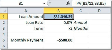
But if we needed to calculate how much we could buy with a $500 monthly payment over a 72 months period at a 5% interest rate? We need to calculate our “present value” (pv), right? For that we have the PV() function:
PV(rate, nper, pmt, fv, type)
As you can see, we could afford to spend as much as $31,046.39 with those conditions.
Another useful financial function is FV(). It can be used to calculate a future value of an investment. Here’s the syntax:
FV(rate, nper, pmt, pv, type)
pv is the present value, or the money that you already have on the investment
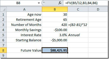
Here’s an example of a retirement plan for a person that is 30 years now, is planning to retire at 65. This will give us a total of 420 monthly payments (35 years * 12 months). He plans to save $100 a month and he will have a 3% annual interest rate on this financial product. He started with a $5,000 deposit.
As you can see, he will have, when he will retire at 65 years of age, $88,425.91 on he’s savings account. If he started without making a deposit, you could omit the pv argument of the function.
Excel has much more financial functions but most of them are aimed to professionals that need to calculate investments analysis, depreciation calculations, etc, they are not aimed for the general Excel user. Maybe later we can see in detail some of them and how you can use them. For now, I hope that you find this basic financial functions useful.


