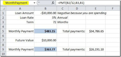
You can use named ranges on your sheets for lots of things. We will see some good examples here on how you can use them. You can name a cell or a range of cells. You can use the name box near the formula bar to insert names on your sheet, just select the cell(s) and type the name you want on the name box, like this:
This will give cell B5 the name “MonthPayment”. Names cannot have blank spaces, special characters, and operators, and can be up to 255 characters long. In this case, to avoid using spaces, I joined the two words but I could use Month_Payment for instance. Now I can just type like this on a cell:
=MonthPayment
and this will display the value I’ve on cell B5. You can use this named ranges to simplify your formulas. For instance, you can now build a formula like this, if you also give cell B3 the name “Term”:
=MonthPayment*Term
As it was explained on the Cascading Validation Lists article, you can also create named ranges using the Name Manager dialog box.
You can use the Named Ranges to navigate through your sheets. Just select the name on the names box on your formula bar and you will jump to corresponding cell(s). This is very useful if you have big and complex worksheets/workbooks.
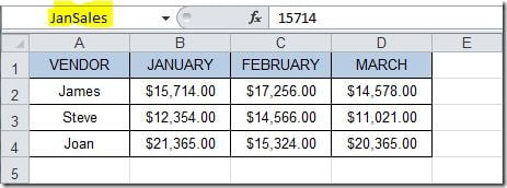
As said before, you can name multiple cells, not just a cell. Let’s see an example on how to do this and how useful this can be. In this sheet, I selected cells B2:B4 and putted a name, on the name box, of JanSales:
Now, I can put a formula on my sheet, for instance on cell B5, just like this:
=SUM(JanSales)
and it will give me the sum of the January sales. It’s easier to read the formulas If you use named ranges!
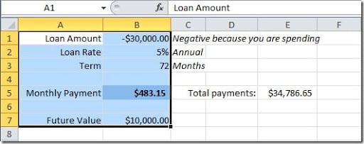
You can create many named cells at once. For instance, with this sheet, just select cells A1:B9 and, on the Formulas tab, on the Defined Names group, click on the “Create from Selection” option.
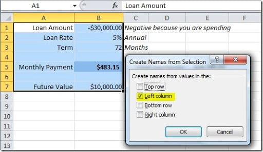
This will open the “Create Names from Selection” dialog box where the “Left column” option is already checked:
In this case, the names that we want to use for our cells are on the left of the values. If they were on the top, with the values below, we would choose “Top row”. Clck the OK button and you will now have 5 names on your name box, one for each value on column B. Excel replaced the blank space by an underscore so that the names can be valid.
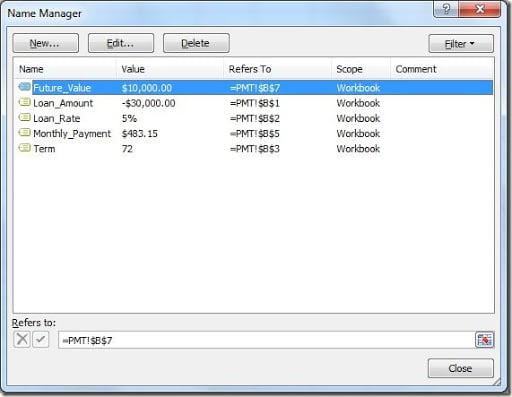
You can manage your names on the Formulas tab, by clicking the Name Manager button. This will open the Name Manager dialog box where you can check the names that you have created, it’s values, the range to where it refers, the scope (either is for the whole workbook or it’s particular to one sheet) and also the comment that you can put to help you identify it. You have also a Filter button that you can use to filter the created names, for instance, if you just want to see the names build for the active worksheet.
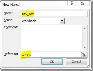
Names can also be used to assign a constant value. Go to Data tab, click on the Name Manager button and on the Name Manager window click on the New button to create a new name. Then create a new name for IRS_Tax and on the “Refers to” field, put a 23% tax value, like this:
Now you can use this constant value on this IRS_Tax name on your formula, like this:
=100*IRS_Tax
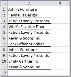
You can created dynamic named ranges. This is very useful if you have a column with data and this column can receive more inputs. This way, you don’t need to edit your named range to the new range, it will automatically adjust it self. Let’s see an example using the OFFSET() function of Excel. We have a list of clients on column A, like this:
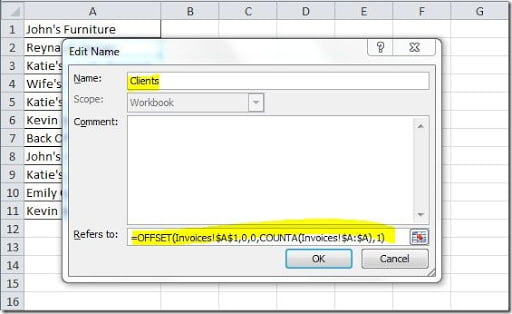
We want to create a dynamic range with the list of clients so that if we had another name on cell A12, the list will expand and consider also this new client name. We will create a new name and on the “Refers to” field, we will put and OFFSET formula, like the one on this image:
After you click OK button, if you click, on the Name Manager window, on the “Refers to” field, you will see that the range A1:A11 is select (with the “marching ants”). Now write a new client name on cell A12 and go to the Name Manager window again to see what range is selected. Is A1:A12, right? As you can see, this is a useful way of creating dynamic Validation Lists.
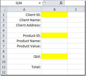
Finally, you can use Named Ranges to help you speed data entry on your sheets! We have seen that you can create named ranges referring to multiple cells. They don’t need to be contiguous cells. Let’s see a vey simple example on how we can apply Named Ranges to helps us speed data entry. We have this simple form:
We just need to insert data on the yellow cells, starting on cell B1, then B5 and finally cell B9. If we want to select a non contiguous set of cells, we just click on the first, then hold down Ctrl key and click on the rest of the cells. If you do this on this three cells, want the name box. It is showing B9 as our active cell. If you put a name for this range on the name box, and then select him on the name box, you will see that your starting input cell will be B9, then it goes to B1 and finally to B5. This is not the order we want! The trick here is to start clicking on our second cell (B5), then B9 and end on the cell that we want to be our first input cell, in this case B1. This is our active cell so this is the one where we should put the name on the name box. So, put for instance, NewOrderInput and press Enter.Now select that name on the name box. You will get all of the three cells selected, starting on B1. Now enter some some value and press Enter. You will see your active cell move from B1 to B5. Repeat the same and you will see it move to cell B9. This is a great way of using Named Ranges to help you improve your productivity when it comes to input data into an Excel sheet.
