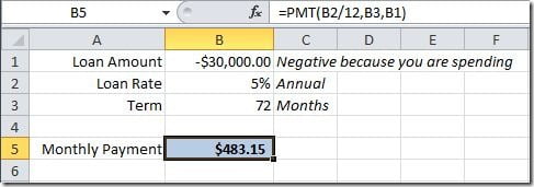
This Excel functionality is very useful when you want to change some input values that give you a final value on a formula. Here’s an example used on our Financial Functions article. We had this formula where we calculate a monthly payment for a certain amount of value, with a certain loan rate, for a certain term:
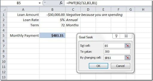
Using the PMT() function, it’s easy to calculate the monthly payment. But we could need to do the opposite. For instance, we know that we can only afford a monthly payment of $300. With the same loan rate and the same loan term, how much money can we ask for? That’s when we can use Goal Seek to calculate the loan amount. Just go to your Data tab, then on the Data Tools group click on the What-If Analysis button and select Goal Seek option. A Goal Seek dialog box opens, like this:
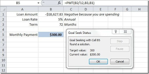
Now we just need to fill the dialog box fields. On the “Set cell” field, we need to select our input cell, in this case is cell B5. The “To value” field is where we are going to put the value our input value, in this case, we want to calculate the loan amount to give us a monthly payment if $300, so fill this with 300. The “By changing cell” field, is where we specify what is the cell that is going to change to give us our final value that we want to calculate, is this case is the loan amount so select cell B1. Just click OK button and we are going to have this result:
As you can see on cell B1, for us to afford a monthly payment of $300, with this loan conditions, we can only ask for $18,627.83. As you can see, this is very easy to use and is a very handy function to have to help us find some particular values.


