 This is a great book from John Walkenbach, also known as “Mr. Spreadsheet”, that will teach you some tricks and will give you great tips on how to do things in Excel 2010. With John Walkenbach's Favorite Excel 2010 Tips and Tricks book you'll get a jump start on mastering the extensive changes to the 2010 version of Excel. This is in my opinion ones of the top books that you should have if you want to master Excel, specially, the 2010 version.
Recommended Book - John Walkenbach's Favorite Excel 2010 Tips and Tricks
Excel 2010–Watch Window
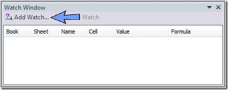
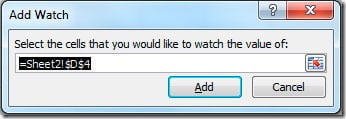
The Watch Window button can be found on the Formula tab, Formula Audition group. Click it and a Watch Window dialog will open. Now click on the Add Watch button in the Watch Window dialog.
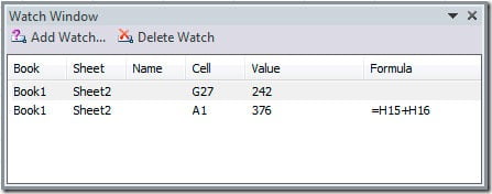
This way you will have a Watch Window that will show you the result of the cells that you’re tracking, without having to switch to the sheet where the formula is to check is result.
Excel 2010 Multithreaded Calculation
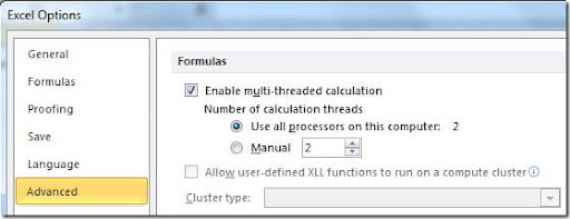
To activate this function, you need to go to File-Tools and on the Advanced category scroll down until you find the Formulas section. Check the “Enable multi-threaded calculation” and select the “Use all processors on this computer”, as shown in this picture.
Evaluate Formulas in Excel 2010
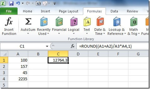
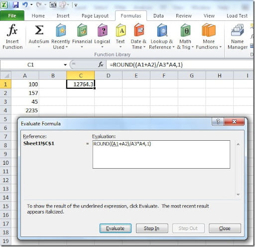
If you select the cell where the formula is and go to the Formulas tab on your menu bar, go to the Formula Audition group and select the Evaluate Formula option, has shown on the image below. This will open a Evaluate Formula dialog box where you can evaluate your formula.
You have an Evaluate button on the bottom that you can click to calculate the underlined portion of your formula (in this case A1). You can use the Step In and Step Out button to go in detail of the underlined portion of your formula.
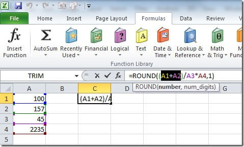
You can also evaluate just a portion of your formula instead of the entire formula. For that, on the formula bar, use the mouse to select the portion of the formula that you want to evaluate. In this example, we just want to evaluate the A1+A2 portion of our simple formula.
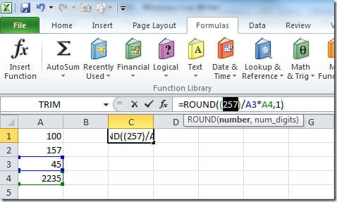
Then press F9 and Excel will just calculate the portion of the formula that you’ve selected, as shown on the next image.
This will display 257 on the formula bar that corresponds to the sum of A1+A2 cell values. Don’t forget to press ESC to exit the formula after you use this method because if you press Enter, that portion of the formula will stay as the calculated value, in this case, it will keep the 257 value instead of the A1+A2 formula.
Recommended Book - Excel 2010 in Depth
 The book that I'm actually reading is Microsoft Excel 2010 In Depth from Bill Jelen. It's a
 The book is divided under 5 main categories:
- Changes in User Interface
- Calculating with Excel
- Business Intelligence
- Visual Presentation of Data
- Sharing
Excel 2010 — Introduction to PowerPivot
- While Excel grid goes until row 1,048,576, has we’ve seen on the Excel 2010 Grid post, with PowerPivot you can handle millions of rows of data. You can sort, filter, scroll and pivot that amount of data using PowerPivot.
- You can create pivot tables with data from multiple tables.
- Import data from different sources like Access, RSS, SQL Server and show the data into a single pivot table.
- DAX — Data Analysis Expressions is the new formula language in PowerPivot. DAX has 117 functions for two types of calculations: 81 normal Excel functions and 54 new functions mainly for data analysis.
- Excel workbooks with PowerPivot are smaller than the ones that use traditional pivot tables.
- You can’t Group on pivot tables.
- You can’t use VBA on PowerPivot as you could with pivot tables.
- PowerPivot can’t be used with other versions of Excel, only the 2010 version.
Excel 2010 — Handling Duplicates
In previous versions of Excel, removing or highlighting duplicates was not a natural thing of Excel, you would need some tricks to do it. Excel 2010 now provides a tool to handle this easily. Take a look at this sample data:
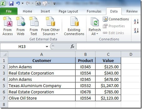
As you can see, there are some Customers and Products duplicated on our table. We want to get a list of unique customers. For that we need to copy the data from column A to another section of our worksheet (in this case the range A1:A7). Then select a single cell within the data set. Go to your menu bar and on the Data tab click on the Remove Duplicates button. A Remove Duplicates dialog box will open like this:
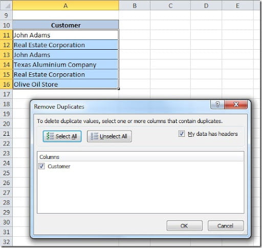
Excel will assume that you have headers on your data and will check the “My data has headers” check box and the name of your columns will appear on the list below. Here is where you will select the fields that you want to make unique records. In this case it’s just the Customer field. Click OK to close the dialog box and you will get a message with the number of duplicates found and remove and the number of unique records that remained.
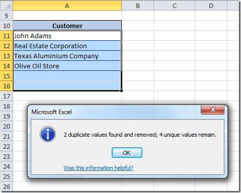
In this example we used just a single column to check for duplicates but we could check for duplicates using more fields. We could check for unique combination of Customers and Product. For that, on the Remove Duplicates dialog box, just select both columns from the list.
Instead of removing your duplicate records, you may want to just highlight them on your sheet so that you can see witch are duplicated. You can do that by using Conditional Formatting option under Home tab. Please check the Highlight Duplicates article for that.
Excel 2010 Grid
In Excel 2003 we had only 65,536 rows and 256 columns. This would gives us 16.7 million cells to work.
In Excel 2010 we now have 1,048,576 rows and 16,384 columns. This more or less 17.1 billion cells on each worksheet witch represents a 102% increase over the old version.
Columns in Excel 2003 where labeled from A to IV. In Excel 2010 they are labeled from A to XFD. This change means that some old range names such as YTD2005 or TAX2006 cannot be used anymore because now they are valid cell addresses. Excel automatically changes this name ranges during conversion. For example, a range name such as YTD2005 will be changed to _YTD2005.
Change the Shape of a Cell Comment
Cell comments is used very often on worksheets but they look always the same way because most users don’t know that they can change the shape of the comment. Instead of being this normal yellow rectangle, it can have lots shapes and colors.
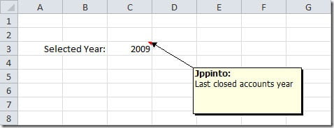
To change the comment shape, make sure that the comment is visible by right-clicking the cell where the comment is placed and choosing Show/Hide Comments options. Then just select the comment border and, in Excel 2003, go to the Draw menu and choose the Change AutoShape option and select the shape you for your comment.

For Excel 2010, you have to add the Change Shape button to your Quick Access Toolbar (QAT). Click on the right arrow on your QAT to open the Customize Quick Access Toolbar, like shown on the picture below. Click on the More Commands option to open the Excel Options dialog window.

On the “Choose commands from” dropdown, select the Drawing Tools Format Tab. On the bottom list, select the Change Shape button and click the Add button. Click OK to close the Excel Options dialog box. Your Change Shape button will appear on your QAT like this:
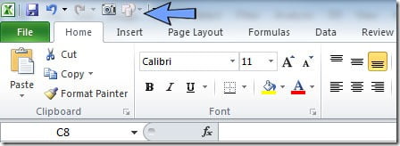
Now that you have your button, you can select your comment border, click on the Change Shape button and select the shape that you want for your comment. the result can be something like this:
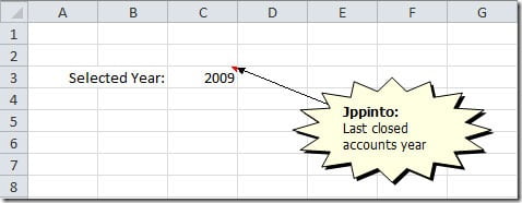
Don’t forget that you can also change the fill color of your comments, the color and weight of your comments border, as well as many other customizations that you can do to your comments for them to stand out on your worksheet.
Excel 2010 — Sparkline Charts
Excel 2010 has a new feature called Sparkline charts that allows you to place a mini-chart inside a cell on your sheet. There are 3 type of sparkline charts: line, column and win/loss. The line and bar charts are very useful to show you a trend about your information while win/loss charts show you positive or negative numbers across a horizontal axis, represented by squares that show positive values if they are above the horizontal axis or negative if they appear below.
To create a sparkline chart, just click on the cell where you want your chart to appear. Click on the Insert tab on your menu bar and click on the type of sparkline chart that you want. A “Create Sparklines” dialog window will appear. The cell that you’ve selected on your sheet will already appear on the field “Location Range” of the dialog window. Click on the “Data Range” field and select on your sheet the range that you want to use on your chart. The range will appear on the “Data Range” field. Click OK and you’re done.
On this picture, you can see on cell F3 a line sparkline chart and on cell G3 a bar sparkline chart.
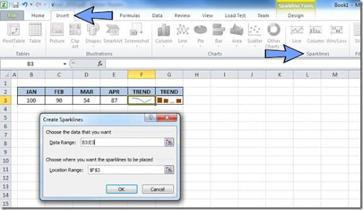
On the next picture, you can see on cell F3 an example of the win/loss sparkline chart.

Excel Camera Tool
Excel has a hidden feature that most of the users don’t know. It’s the Camera Tool. For Excel 2003, you can get the button for the Camera Tool by going to Tools-Customize, on the Commands tab, find the category Tools. Scroll down until you find the Camera button. Drag and drop the button into one of your toolbars. Close the customize dialog window.
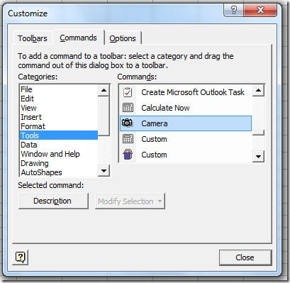
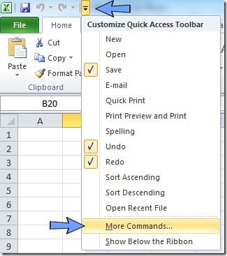
For Excel 2010, you need to make the Camera button appear on the Excel Quick Access Toolbar. Go to Quick Access Toolbar, click on the drop down button and select More Commands, like on the picture below:
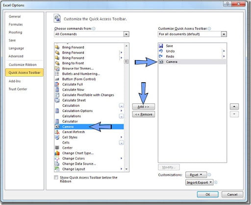
This will open Excel Options dialog box. On the “Choose commands from” drop down select “All Commands” to see all Excel commands. Scroll down the list until you see the Camera command. Select it from the list and click on the Add button on the right. Once it appears on the right box, click OK button from the dialog box.
Your Camera button will appear now near the drop down button on your Excel Quick Access Toolbar:
Now that you have the Camera Tool button available, let’s see what you can do with it. This tool can be very useful if you want to display a part of your sheet on another location, without affecting the formatting of that area. Let’s see a practical example. Suppose I have the following table:

I want to show this table on a chart. For that, I will “take a picture” of the table from one of the sheets and place the “picture” on top of the chart that I have on another sheet. Just select the table cells and click on the Camera tool button on your toolbar. Then on the sheet that has the chart just click on one cell and the “picture” of your table will be displayed like if you have inserted a picture on your sheet. You can now work this “picture” the way you want it to look and place it on top of your chart. The final result will be something like this:
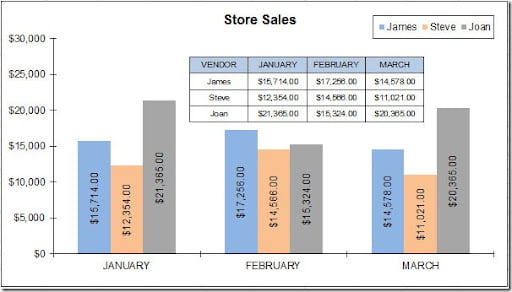
This tool is very useful if you want to display tables from different sheets without having to adjust the formatting of the target sheet.
Highlight duplicates
One of the most common tasks that an Excel user needs to do is to find duplicates on a list of data. There are several ways to do this, depending on the needs. One of the ways is to highlight the values that are duplicated on a column. This can be done using the Format-Conditional Formatting option on the menu bar. Here's an example:
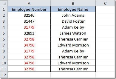
On cell A2, I created a Conditional Formatting with a condition "Formula is" and putted the function =COUNTIF(A:A,A2)>1. The COUNTIF function has the following syntax:
COUNTIF(range,criteria)
range is the area where you you want to check if it finds the value specified by criteria.
This will return TRUE if the value from cell A2 is found more than 1 time in column A. If this is TRUE it will apply the Format that I defined. I then Copy and Paste Special-Format to the rest of the cells in column A.
In Excel 2007 and 2010, you can use the a new option on the Conditional Formatting menu that is the Duplicate Values.
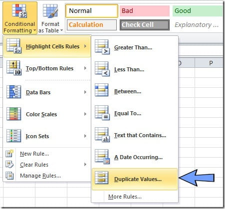
Just select the range where you want to highlight the duplicate and go to the menu bar and choose Highlight Cells Rules-Duplicate Values. A Duplicate Values dialog box will open. You can choose to highlight the Duplicate or the Unique values and you can set the color that you want to use to highlight the values.
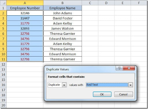
The result will be the same as using the COUNTIF solution. On Excel 2003 you don’t have this Duplicate Values option on the Conditional Formatting menu.
