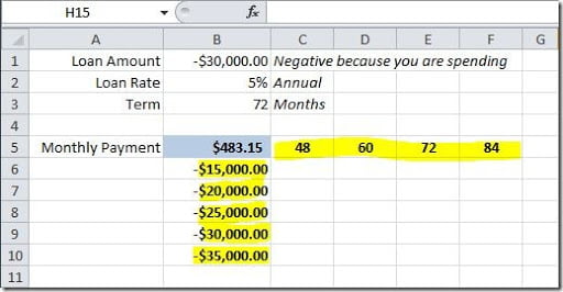
Sometime ago, I wrote an article about Financial Functions in Excel. Using the PMT() function, I wanted to calculate a monthly payment for a loan, during a certain amount of months, at a specific interest rate. It looked something like this:
But what if we wanted to calculate the monthly payment using different loan terms? For instance, for 48, 60 and 84 months, instead of only 72? Sure, we could change the value on cell B3 and check the value for each term or we could copy the formula for each of the term value to see how it would change the monthly payment, but, what if we wanted also to check the monthly payment value if, not only we changed the loan term but also the loan amount? Excel has an easy solution for that! It’s called What-if and can be found on Excel 2010 on the Data tab, on the Data Tools group. Let’s see how we could use it to solve our problem.
Let’s put on column B the loan amounts that we want to use on our simulation and on row 5 the number of months for the term of our loan, like this:
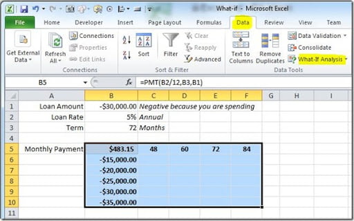
Now we want to fill the rest of this table with the calculation using the formula on cell B5. This is where What-if function get’s in to action. Select your table (range B5:F10), Go to Data tab, and click on the What-If Analysis option. Then select Data Table.
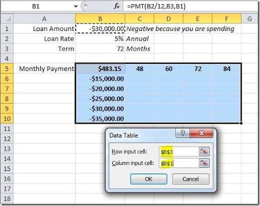
A Data Table dialog box will open. On the “Row input cell”, we want the values on the top row of our table (range C5:F5) to the the input for our loan Term, so we should set this to cell B3. On the “Column input cell”, we want the values on our left most column of our table (range B6:B10) to be the input of our Loan Amount, so we should set this to cell B1, like this:
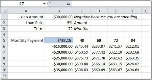
Click OK button and your will get your data table filled out showing the monthly payments for the loan, with the different loan terms and loan amounts, like this:
As you can see, this is easier than copying the formula to multiple cells or changing the values on the original formula to check what happens if you change any variable.


